
Upzoning
When zoning constrains housing supply, upzoning leads to more homes

In 2015, the city of Auckland had roughly 350,000 units of ‘zoned capacity’: homes that could theoretically be built under the existing zoning. So you would expect that adding more zoned capacity would have no effect, like pushing on a string. And yet, after Auckland upzoned in 2016 to allow townhomes and apartments, housing construction surged, leading to a substantial increase in the housing stock. How did upzoning kick off a construction boom, if their zoning already allowed more than enough new supply?
The answer is that Auckland’s pre-reform zoned capacity was largely theoretical. Much of it required redevelopment that was not economically feasible at prevailing prices and construction costs. Their upzoning worked because it created feasible capacity: projects that developers could profitably build right away. The payoff from this increase in housing supply was a decrease in rents compared to other cities.
More generally, zoning constrains housing supply when developers want to build at a higher density than the zoning allows. For example, if zoning allows only detached houses where developers would otherwise build six-storey apartments, then zoning is preventing supply from keeping up with demand. Upzoning relaxes the zoning constraint and increases the supply of housing. Since increasing supply leads to lower prices, upzoning is a key policy option for improving housing affordability.
Upzoning reduces land costs and raises land prices
Upzoning increases the supply of high-density land, for example, by converting land zoned for detached houses into apartment-zoned land.1 So to understand upzoning, we need to look at its effects on the land market. Upzoning has seemingly contradictory effects: it reduces land costs per home, while increasing the price of land per parcel.
Upzoning a parcel of land reduces land costs by reducing the physical amount of land required to build a home. When zoning allows one house per parcel, you need to buy a whole parcel to get one home. But if the zoning allowed six apartments on a parcel, you now only need to pay for one-sixth of the parcel. So upzoning allows you to save on land costs by splitting the cost of land over more homes.
But doesn’t upzoning increase the value of the upzoned parcel itself? Most likely, yes. An apartment building generates more revenue than a single house, so developers are willing to pay more for apartment-zoned land. But this is consistent with a decrease in land costs: even though the parcel is more valuable when zoned for higher density, the land cost per home still decreases.2
For example, suppose that a vacant parcel zoned for a single-family house has a land price of $1M; when we upzone for a six-unit apartment building, developers bid more, so the land price rises to $3M. But the land cost is now split across six units, so the land cost per home falls from $1M / 1 = $1M per house to $3M / 6 = $0.5M per apartment.3 As we’ll see below, this is what happens in practice.
Upzoning also has the effect of reducing the price of existing high-density land. Imagine you own a vacant parcel of land zoned for apartments. When zoning restricts apartments across the city, developers are prevented from building, so they bid up the price of apartment-zoned land. This adds a scarcity premium to your land, making it artificially expensive. So when another street is upzoned for apartments, developers build them and increase the housing supply; this lowers rents, which reduces how much developers are able to bid for your land.4
So upzoning reduces land costs per home and has opposing effects on land prices, depending on which land we’re talking about. It increases the price of the upzoned parcel, by allowing more-valuable uses for which developers will pay more. And it decreases the price of existing high-density land, by increasing housing supply, reducing rents, and reducing developers’ budget for land.
When is zoning a constraint on housing supply?
How do we know when zoning is a constraint on the supply of housing? The simplest test is to change it and see what happens: if we upzone a parcel to allow higher density, do developers build more homes there? If so, then zoning was a constraint on supply. If upzoning doesn’t lead to any long-run changes in behavior (holding other factors constant), then it wasn’t a constraint.
Land values are another signal of restrictive zoning. Is land zoned for high-density more expensive than land zoned for low-density (controlling for location)? This gap is the scarcity premium created by restrictive zoning, and upzoning should decrease it. We can also look at whether upzoning a parcel increases its land price: are developers willing to pay more for land with more valuable uses? If so, then zoning is making high-density land artificially scarce.5
Another test of constrained zoning is whether new housing is built right up to the density limit; if zoning limits density, developers will build near the maximum allowed. More practical signs of restrictive zoning include developers requesting variances or rezonings, and NIMBY activists fighting to prevent upzoning: if zoning didn’t have any effect, they wouldn’t care if it was changed.
What would a city with unconstrained zoning look like? Developers building single-family houses on apartment-zoned land. When there’s enough upzoned land that developers can meet all of the demand for apartments, they will use the remaining land to build houses. As long as new projects in an apartment-zoned area are consistently built as apartments, we know that we don’t have enough land zoned for apartments. Alternatively, zoning is unconstrained when upzoning one additional parcel does not increase its land value, because developers are not willing to pay more for high-density land; the scarcity premium is zero. This also implies that low- and high-density land prices should be equal (controlling for location), since there’s no scarcity premium on high-density land.
When zoning constrains development in the city, it pushes new housing out into the suburbs. This forces people to either double-up with roommates in the city, or live in the suburbs with a long commute. Upzoning to allow more density in the city reverses this, allowing more people to live near their job and family. Hence, restrictive zoning may not change the metro-wide stock of housing, but it does distort supply by preventing people from living in desirable locations.
Zoned capacity: feasible or infeasible?
Returning to Auckland, if the 2015 zoning allowed developers to build 350,000 additional homes, why did they upzone to allow more? ‘Zoned capacity’ is the difference between the total housing stock theoretically allowed under current zoning and the existing housing stock. In economic terms, this is the housing supply that developers would produce if prices were infinitely high.6 But housing that will be built when rents reach $7000 is simply not relevant. What we care about is capacity that can be built right now.
The reason zoned capacity can be meaningless is redevelopment costs. Suppose a parcel has an existing 3-storey apartment and we upzone to allow for a 5-storey building. According to zoned capacity, there are now two floors of housing waiting to be built. But this requires paying demolition costs; a developer would tear down a 3-storey building to rebuild at five storeys only when prices are very high. The upzoning didn’t create feasible zoned capacity that can be profitably built at current prices.
Hence, a large zoned capacity does not imply that developers will produce a large quantity of housing at current prices. The 350,000 units of zoned capacity in Auckland were not all feasible to build. Their upzoning led to a construction boom that reduced rents because it created feasible zoned capacity.
So the theoretically-allowed housing stock is not relevant for policy. Instead, we need to ask: how much housing will be produced at what rent level? And we should evaluate a proposed upzoning based on how much feasible zoned capacity it adds.
Evidence from large upzonings
It’s important to study large upzonings that increased density by a substantial amount, since this allows us to test whether upzoning has an effect. If you take a tiny dose of medicine, you can’t learn whether the medicine actually works. Similarly, a small upzoning that barely changes zoning laws or is counteracted by poison pills (regulations that undermine feasibility) is not informative. We want a large policy change that will generate statistically-detectable effects. Luckily, we have two case studies of large upzonings: Auckland and São Paulo.
But first, we need to define one acronym: floor area ratio, or FAR, is the ratio of a building’s total floor area to the area of the land it sits on. At FAR=1, a 1-storey building could cover the entire lot, or a 2-storey building could cover half of the lot. For a building that covers half of the parcel, an extra 0.5 FAR allows you to build one storey taller.
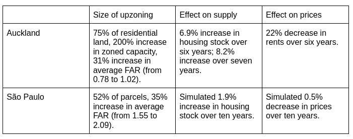
Auckland
Auckland is the largest city in New Zealand. In 2016, it upzoned three quarters of its residential land, tripling the city’s zoned capacity, and raising the average maximum FAR by +0.24 from 0.78 to 1.02 (a 31% increase).7 The Auckland Unitary Plan (AUP) changed the zoning from primarily single-family houses to higher-density zones allowing triplexes, townhomes, and mid-rise apartments.8 Importantly, the upzoning increased both the number of allowed units as well as the maximum density; many zoning reforms fail by allowing more units per parcel without increasing density, which means the homes must be smaller and hence lower quality.
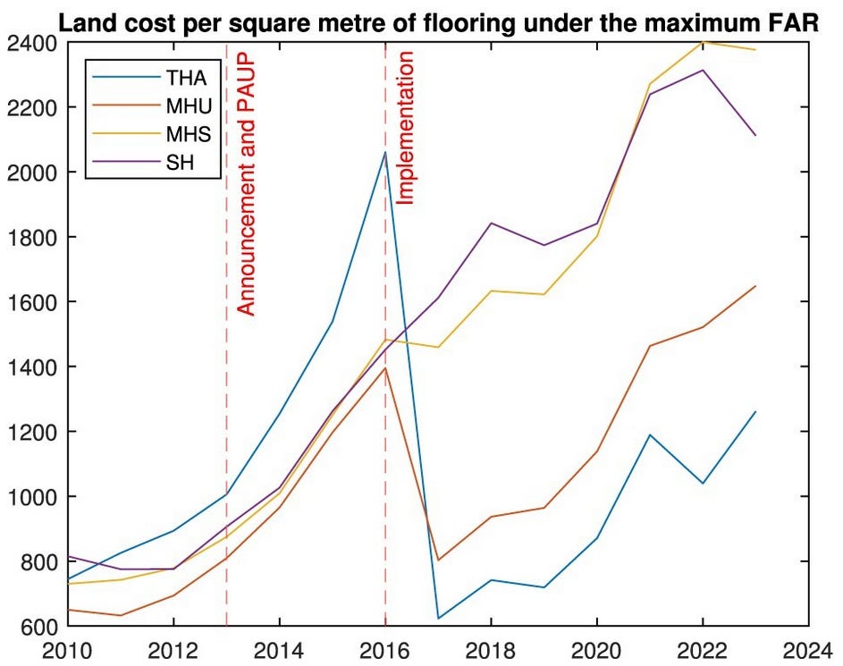
The four zones under AUP are9:
Terrace Housing and Apartment Buildings (THA): 5-7 storeys, 2.5 FAR, no dwelling limit.
Mixed Housing Urban (MHU): 3 storeys, 1.35 FAR, 3 dwellings.
Mixed Housing Suburban (MHS): 2 storeys, 0.8 FAR, 3 dwellings.
Single House (SH): 2 storeys, 0.7 FAR, 1 dwelling.
Was zoning a binding constraint in Auckland? Yes. First, as we’ll see below, upzoning led to a construction boom; if zoning was not binding, there would be no effect on supply. Second, the price of land in upzoned areas increased relative to non-upzoned areas.10 This implies that developers were willing to pay more for land that allowed higher-density housing. If zoning was not a constraint and extra density had no value, then land prices would not change.
Did upzoning reduce land costs? We have direct evidence from Cooper, Greenaway-McGrevy, and Jones (2025), who calculate land cost per square meter of floorspace as land prices divided by floorspace; see their Figure 3c plotted below. Land rezoned to the apartment category (THA) had high and increasing prices before 2016. When the reform was implemented, upzoned land gained valuable new development rights and land prices rose. At the same time, the maximum FAR increased from 0.7 to 2.5, so the allowed floorspace rose by a factor of 3.6. On net, the effect was a sharp decrease in land cost per square meter.11
What happened to housing supply? Greenaway-McGrevy and Phillips (2023) (working paper, published) studies Auckland’s upzoning using housing permits, the number of homes approved for construction. They compare upzoned areas, which allowed townhomes and apartments, to non-upzoned areas that remained limited to detached houses. If permits increased more in upzoned areas relative to non-upzoned areas, then we can attribute that extra construction as an effect of the upzoning.
The upzoning worked as predicted: most of the increased permits came from attached dwellings (e.g. townhomes and apartments) rather than detached houses (Fig. 3), and they were mostly located inside the urban core rather than outside (Fig. 4). The increase in permits in the highest-density zone came entirely from attached dwellings, while the lower-density zones saw a mix of attached and detached. This shows that high-density zones are used for higher-density housing.
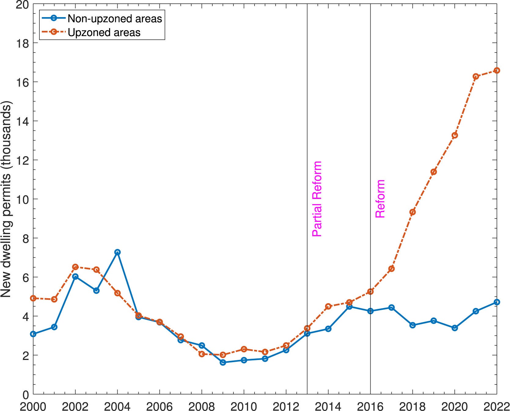
Overall, upzoning led to a big increase in housing supply in upzoned areas, as shown in the graph above. This indicates that restrictive zoning was preventing people from living near transit and jobs downtown.12 Hence, the effect of upzoning is to increase housing supply in the places where people want to live.
We also expect that upzoning enabled people to have more personal space, e.g., moving out on their own instead of living with parents or roommates. Future research should study where the residents in upzoning-induced housing came from. Did they move in from the suburbs, or were they already living doubled-up in Auckland?
Increased supply in upzoned areas raises the question: did upzoning merely reallocate new construction to more desirable locations, or did it also increase the overall housing stock?13 The authors show that most of the new construction was a net increase, with some new housing being displaced from the non-upzoned areas to the upzoned areas.14 So upzoning didn’t just reallocate homes to better locations, it also increased the housing stock. This suggests that upzoning enabled in-migration from outside of the Auckland metro area, and allowed for household formation, with roommates undoubling and adult children moving out on their own.15
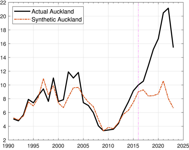
Greenaway-McGrevy (2026) also studies construction in Auckland, this time using the synthetic control method. This approach creates a composite version of Auckland that was never upzoned, which we can use as a control group for the real Auckland.16 So to get the effect of upzoning, we simply compare synthetic-Auckland to real-Auckland (see Fig. 6b, shown below). With this approach, Greenaway-McGrevy estimates that upzoning increased permits by about 52,000 (or 87%) over seven years, relative to the control group.17 So the latest evidence implies an 8.2% increase in the net housing stock.18
Since upzoning caused a large increase in permits, these two papers give strong evidence that zoning was a binding constraint on housing supply in Auckland. And for such a large increase in supply, we expect to find a decrease in housing rents. This is studied in Greenaway-McGrevy and So (2024) (working paper), using data on quality-adjusted rents over 2000-2022.19 They also use the synthetic control method, constructing a synthetic Auckland from other cities in New Zealand. In preliminary results, they find that after six years, upzoning decreased rents by 22% relative to the control group. In other words, without upzoning, rents would be 28% higher than they actually are.20 Auckland rents still rose in absolute terms after 2016, so the reform wasn’t a panacea; but rents would have increased even more without upzoning.
Hence, Auckland shows us how upzoning works. Since zoning was a constraint, allowing more homes led to increased housing supply, reduced land costs per home, and ultimately led to lower rents. Putting the causal results together, we get an elasticity of rents to housing stock of -3.6: a 1% increase in housing stock reduces rents by 3.6%.21 We can use this elasticity to infer that if upzoning had increased the housing stock by 12% over six years (instead of the actual 6.9%), then rents would have stayed flat.22
São Paulo
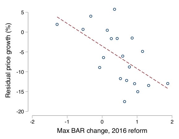
São Paulo is the largest city in Brazil, with a population of 11 million and a metro population of 22 million. Anagol, Ferreira, and Rexer (2023) (working paper) studies the effects of São Paulo’s 2016 zoning reform, which changed allowed density on a block-by-block basis. Allowed density increased on half of city blocks, driven by increased FAR along public transit routes, though some central areas were downzoned.23 On average, the maximum allowed FAR increased by 35% (or 0.55 FAR points, from 1.55 to 2.09). The authors use the fine-grained zoning map to test how upzoning affects permitting, construction, and prices. As we’ll see, upzoning increased housing supply, so zoning was a binding constraint.24 But even though the São Paulo upzoning was larger than Auckland’s in percentage terms, it actually had a smaller effect on housing supply.
To study the effects of upzoning on permitting and construction, the authors compare blocks on opposite sides of zoning boundaries. On the upzoned side, FAR is increased and developers can build at higher density; on the other side, the allowed density was unchanged or decreased. The key idea is that these blocks are very close to each other, so they are similar in many ways, sharing the same neighborhood, amenities, jobs, and transit; comparing nearby blocks helps isolate the effect of upzoning. Then the authors ask: after the 2016 reform, did permitting and construction increase more on the upzoned side compared to the non-upzoned side?25
Anagol et al. find that a 1-point increase in FAR leads to a 28 to 63% increase in multifamily permits filed, relative to control blocks. Approved permits increased even more, by 47 to 88%; this suggests that upzoning increased the approval rate. They measure new supply using property listings, and find that upzoning led to 2.1 additional listings (or a 10.3% increase) in treatment blocks relative to control blocks. Hence, upzoning led to more permits being filed and approved, and more homes being constructed and listed for sale.26
To study the effect of upzoning on prices, we need a different method. Prices are determined by supply and demand across the entire market, so increased supply in one block will reduce prices in the neighboring block as well, making it unsuitable as a control group. To address this, the authors use entire neighborhoods to measure separate housing markets; they divide São Paulo into 329 neighborhoods, each with roughly 10,000 households. The assumption here is that increases in housing supply in one neighborhood do not affect prices in other neighborhoods.27
Using neighborhood-level data, we can compare the change in quality-adjusted prices from 2019 to 2022 to the change in average FAR due to upzoning. They find that a 1-unit increase in FAR is associated with a 5.7 percentage point decrease in housing price growth.28 Their Figure 6 (see below) shows that neighborhoods with increased density have lower prices (i.e., negative price growth), and that larger density increases correspond to larger decreases in price growth.
The authors also estimate a structural model, which allows them to run a ten year simulation. They estimate that the 2016 reform would lead to a 1.9% increase in the housing stock over ten years (47,000 new units over a base of 2.45M), compared to the status quo. This leads to a 0.5% decrease in housing prices, a result that is partly driven by modelling assumptions.29
They also evaluate a counterfactual ‘double upzoning’ reform that increases average FAR from 1.55 to 3.49; this is a 125% increase in allowed density compared to the actual 35% increase under the 2016 reform. The ‘double upzoning’ would lead to a 27.5% increase in housing stock (678,000 new units) and a 7.5% decrease in prices. Hence, the effect of upzoning on housing supply is strongly nonlinear: a 3.6x larger increase in allowed density leads to a 14x larger increase in housing stock.30
Discussion
In Auckland, a 31% increase in allowed FAR (from 0.78 to 1.02) led to an 8.2% increase in housing stock over seven years. São Paulo increased FAR by 35% (from 1.55 to 2.09), but we expect only a 1.9% increase in housing stock over ten years. What’s going on? One possible explanation is that São Paulo’s nominal increase in FAR was undermined by poison pills like height limits, shadow regulations, or inclusionary zoning.
A different explanation is that Auckland’s zoning was more stringent, and that São Paulo had a smaller supply effect because its upzoning actually eliminated the scarcity premium (the gap in land price between similar high- and low-density parcels). With data on land prices, we could test whether the scarcity premium before upzoning was larger in Auckland than in São Paulo, and whether it was reduced to zero in the latter. But the bigger supply effect from the ‘double upzoning’ cuts against this explanation: further upzoning would have an effect only if zoning remained a constraint.
A better explanation is based on redevelopment costs. Auckland’s existing housing stock was mostly detached houses, while São Paulo had more apartments. Since houses are cheaper to demolish and redevelop than apartment buildings, applying a similar density increase to both cities led to much bigger effects in Auckland. Similarly, the stronger effect from ‘double upzoning’ suggests that higher allowed densities are needed to overcome redevelopment costs in São Paulo–they didn’t upzone enough.
So after adjusting for redevelopment costs, we can say that Auckland had a larger effective upzoning, since it led to a bigger increase in feasible zoned capacity: housing supply that can profitably be built at current prices. In contrast, São Paulo seems to have added more infeasible zoned capacity that is currently unprofitable to build.31 This shows that not all upzonings are equal, because not all zoned capacity is equal. When existing buildings are costly to redevelop, increasing allowed FAR may not translate to an increase in feasible capacity.
Other upzonings
Maltman and Greenaway-McGrevy (2025) studies another upzoning in New Zealand, this time in Lower Hutt, a municipality in the Wellington metro area. Lower Hutt implemented a sequence of reforms over 2016-2023: reducing and then removing parking minimums, a limited upzoning allowing small apartments and townhomes, and a widespread upzoning allowing larger apartments and townhomes. Overall, FAR increased by +1.04 or 141%.32 The authors use a synthetic control method, and report a 10-22% increase in metro-wide housing permits after six years, or a 0.9%-1.4% increase in the net housing stock, accounting for construction being displaced from non-upzoned areas.33 Looking at quality-adjusted rents, they find that upzoning reduced rents by 17% compared to the synthetic control group.
Rollet (2025) (working paper) studies a sequence of upzonings in New York City. These mostly occurred over 2005-2010 during the Bloomberg administration, and upzoned 6% of parcels. On average, upzoning increased allowed floorspace by 61%.34 Comparing earlier- and later-upzoned parcels, Rollet shows that a 1-point increase in maximum FAR is associated with a 0.09 increase in built floorspace after ten years. Again, this is explained by redevelopment costs: since NYC is already built-up, redevelopment occurs slowly due to fixed costs from demolition.35 As a result, redevelopment is more likely in low-density neighborhoods where prices are high, since these have low demolition costs and high returns. Rollet’s study is not designed to estimate the effect of supply on rents, since rents are determined by the metro-level housing supply, and he doesn’t have a control group for metro NYC.36
Büchler and Lutz (2024) studies a sequence of upzonings in the Canton of Zurich over 1995-2020. Most municipalities relaxed their zoning, with the typical reform increasing allowed floorspace by 31%. To estimate the effect of upzoning on housing supply, they compare earlier-upzoned areas to later-upzoned areas.37 The authors report that, after ten years, upzoning increases both floorspace and the number of housing units by 9%.38 They find larger effects for larger upzonings and where zoning was binding.39 As with Rollet, this study is not designed for estimating an effect on rents, since rents are determined by supply and demand at the metro level, and they don’t have a control group for metro Zurich.
These examples reinforce the lesson that upzoning works when it creates economically feasible housing supply, with enough new density to overcome redevelopment costs. Some limited zoning reforms have had limited effects. Chicago introduced discretionary transit-oriented zoning in 2013 and 2015, but did not actually upzone to allow higher density (i.e., by-right zoning). Minneapolis allowed three units per parcel in 2020, but without increasing allowed floorspace, so the new homes had to be smaller. These reforms did not create feasible zoned capacity.
Conclusion
Zoning has become a constraint on housing supply in cities around the world, making upzoning a key policy tool for improving housing affordability. We can detect when zoning is a binding constraint by looking for a scarcity premium in the price of high-density land, such as land in an apartment zone being more expensive than otherwise similar land in a house zone. When zoning is a constraint, upzoning increases land values; we’ll know that zoning has stopped being a constraint when high-density land is no longer scarce and upzoning has no uplift effect on the parcel’s land value. In this world, apartment-zoned land will sell for the same price as otherwise similar house-zoned land, and developers will build houses in apartment zones. Cities should continue upzoning until the zoning constraint stops binding.
Upzoning increases the allowed density on a parcel of land. This can be: urban growth boundary expansion (converting from agricultural to residential), reducing minimum lot size (allowing more houses on the same land area), or increasing height and density limits (converting from single-family houses to six-storey apartments). Upzoning is additional in the sense of adding new uses without changing the original use; you can still build a house on apartment-zoned land.
We can also measure land costs per square foot of floorspace of housing.
It’s possible for upzoning to decrease the value of the upzoned parcel: when housing prices drop so much that the return to building high-density housing is lower than the initial low-density value.
E.g., a SFH sells for $2M and construction costs are $1M, so the residual land value is $1M. Each apartment sells for $1M and costs $0.5M, so the residual land value is $0.5*6 = $3M.
What if apartments had the same price and cost as houses? Then the land value would rise proportionally with density, and land cost per home would be constant. This is the limiting case, corresponding to perfectly elastic demand and constant marginal costs.
This is the capitalization of lower housing prices into the price of existing high-density land. This ‘cross-parcel’ effect is visible only when there already is some apartment-zoned land; if you’re upzoning for the first time, then there is no high-density land to make cheaper. Here we just have the direct effect on land cost per home. Similarly, when zoning is discretionary instead of rules-based, as in Vancouver, then there is no existing apartment-zoned land to affect.
Another metric is the Glaeser-Gyourko ‘zoning tax’ comparing the price of housing to the marginal construction cost. When zoning is a constraint, it creates a wedge between price and marginal cost, where developers can build new homes at a marginal cost below the market price. This wedge is the scarcity premium embedded in higher-density land prices. See Gyourko and Krimmel (2021).
Formally, it is the housing supply curve Q_S(P) evaluated at infinite prices: Q_S(∞).
Zoned capacity: “Prior to the AUP, with infill and redevelopment there was estimated capacity for 345,176 additional dwellings [...] After the AUP, this figure was 1,076,267.” fn4, Greenaway-McGrevy, Pacheco, and Sorensen (2021).
FAR: using the data on land areas in Table 1 from Greenaway-McGrevy and Jones (2025) for the four residential categories (excluding business and rural), and assigning the midpoint FAR for the pre-AUP categories, we get pre-reform average FAR as 0.15(2.5)+3.58(1.925)+9.10(1.075)+273.67(0.75) / 286.50km2 = 0.78 FAR. Post-reform average FAR is 21.27(2.5)+63.21(1.35)+132.94(0.8)+69.08(0.7) / 286.50 km2 = 1.02 FAR.
Alternatively, using the parcel-level data in Table 2 from Cheung, Monkkonen, and Yiu (2024), we calculate the pre-reform average FAR as (159172*0.70 + 18109*0.80 + 24659*1.35 + 1880*2.50)/203820 = 0.80. Average post-reform FAR is (54242*0.70 + 88281*0.80 + 47956*1.35 + 13341*2.50)/203820 = 1.01. So calculating average FAR using parcels instead of land areas gives very similar estimates.
A draft upzoning plan was published in 2013, with the actual policy implemented on November 15, 2016, so there may be anticipation effects before 2016. There was also an inclusionary zoning policy in Special Housing Areas starting in 2013.
Greenaway-McGrevy and Phillips (2023) shows that land prices increased by 25% in upzoned areas, starting in 2014; see Figure 22. Cheung, Monkkonen, and Yiu (2024) also reports 6-13% higher assessed property values in upzoned areas; see Table 4. Greenaway-McGrevy, Pacheco, and Sorensen (2021) shows that land values increased more in higher-density zones; see Table 2.
We also expect that before AUP, higher-density land was more expensive due to its supply being artificially restricted by zoning. I haven’t seen data on this.
2.5/0.7 = 3.6. This is relevant if developers actually built up to the 2.5 FAR limit; if they build only to 2.0 FAR, say, then we need to divide by 2.0 instead of 2.5. I haven’t found any data on built FAR.
We should also be able to show that high-density land prices decreased. For example, there were 389 THA parcels with unchanged zoning status after AUP. Since the THA category increased by 11,000 parcels, we expect this influx of competition from new THA landowners to increase supply and reduce rents, thereby decreasing how much developers will bid for the initial 389 parcels. However, no one has run this analysis (yet).
Greenaway-McGrevy and Jones (2025) shows that new housing is located closer to the central business district, job centers, and rapid transit stations.
In the closed-city/fixed-population version of the monocentric city model, upzoning allows more people to live closer to the city center, without changing the total number of dwellings. This model doesn’t allow for household formation or in-migration. Even though the housing stock is unchanged, housing prices fall because higher-density housing reduces land costs per home. See Cooper, Greenaway-McGrevy, and Jones (2025).
They extrapolate construction trends in the control group to figure out how much construction would have occurred in the non-upzoned areas in the world where the upzoning didn’t occur. Then we compare the upzoned areas to the predicted trend in the non-upzoned areas, where the difference captures the net effect of upzoning accounting for displacement.
They estimate a net increase of roughly 22,000 homes permitted over five years, which translates to a 3.4% increase in Auckland’s net housing stock. In an updated paper, Greenaway-McGrevy reports a net increase of roughly 34,000 permits over six years (for a 5.4% increase in the housing stock).
3.4% over five years: 21808 * 0.94 * 0.89/530000 = 0.034. Assuming a 0.94 completion rate and a 0.11 demolition rate, assumptions taken from Greenaway-McGrevy 2025.
5.4% over six years: 34064 * 0.94 * 0.89/530000 = 0.054. Greenaway-McGrevy (2023) extends the sample by one year and uses a slightly different specification. As robustness checks, he includes business and rural zones in the control group, and analyzes the inclusionary zoning program started in 2013. Donovan and Maltman (2025) rebuts criticisms of Greenaway-McGrevy and Phillips (2023).
Note that increased in-migration implies that housing construction decreased in the origin cities of the migrants. Only household formation unambiguously increases the aggregate housing stock.
We construct the synthetic control group as a weighted average of other non-upzoned cities. Are other New Zealand cities an appropriate control group, if they can be affected by Auckland’s upzoning? For example, new housing in Auckland could induce migration or shift construction labor from other cities, which would bias the treatment effect upwards. There could also be a downward bias, if redevelopment involved trucking old houses over to the control cities (instead of demolishing them). Greenaway-McGrevy tests for such spillover effects by creating a synthetic control for each of the control cities; he finds no evidence of spillovers.
How do the two methods compare? Using the synthetic control method, upzoning caused about 43,500 additional permits over six years (eyeballing Fig 6b, there were 8700 permits in 2023, which we subtract from the 52200 total over seven years). In the updated difference-in-differences paper, this was 34,000 over six years. This suggests that the difference-in-differences analysis is overly conservative in using non-upzoned areas in Auckland as the control group.
52000 * 0.94 * 0.89/530000 = 0.082.
They use a hedonic rent index, accounting for number of bedrooms, housing type, and location.
E.g., decreasing rents from 100 to 78 implies that reversing the policy would increase rents from 78 to 100, which is a 28% increase. Or: (100-78)/78 = 0.28.
The elasticity of rents to housing stock is ln(1-0.216)/ln(1 + 0.069) = -3.6. Over six years, rents fell by 21.6% (Greenaway-McGrevy and So 2024) and the net housing stock increased by 6.9%. The gross increase was 43500 units over a base of 530000, which falls to 36347 after accounting for a 0.94 completion rate and a 0.11 demolition rate; and 36347/530000 = 0.069 (Greenaway-McGrevy 2025).
Graphically, the rent-to-supply elasticity is from shifting the supply curve while demand is held fixed. Hence, we need the causal estimates of effects on rent and supply. Just using the observed changes in rent and supply doesn’t hold demand fixed, and doesn’t tell us the rent-to-supply elasticity.
Actual rents increased by 18.1%, so to hold rent growth at 0%, we need additional supply growth x: ln(1.181) = 3.6*ln(1+x), which gives x=0.047. So the housing stock needed to grow by 1.069*1.047 = 1.12.
Density increased in 52% of city blocks, and was unchanged or decreased in the remaining 48%.
They don’t use their data on land values to measure how stringent zoning constraints were before 2016, or whether upzoning reduced high-density land prices.
This is a boundary regression discontinuity approach, where we compare the treatment-control difference at the zoning boundary after 2016 to the treatment-control difference at the boundary before 2016.
The authors test for displacement of construction from control to treatment blocks, and do not detect a displacement effect.
It’s plausible that upzoning in one neighborhood does have spillover effects on other neighborhoods. In this case, higher housing supply leads to lower prices in the control group, so the treatment effect is underestimated; the actual effect on prices is even larger than what they report.
They don’t have price data before 2019, so can’t test for differential pre-trends. Since upzoning is not randomly assigned, it’s possible that neighborhoods with falling prices were assigned larger upzonings. Table A9 includes subprefeitura fixed effects, and the effect on price growth falls to -3.2pp. (Note that this is a regression in differences, so subprefeitura FEs are equivalent to subprefeitura-year FEs in levels.)
The model assumes that prices are determined by housing supply in the city relative to supply in the suburbs. It also assumes that the suburban housing stock grows at a fixed rate. Combined, these assumptions mute the effect of upzoning on prices. But since high suburban growth is an outcome of restrictive zoning in the city, we would expect upzoning to actually reduce suburban growth. This is not allowed in the model.
They also assume that vacancies created by new supply are filled by migrants (from outside the metro or from the suburbs). This means upzoning is reducing demand and prices in the origin neighborhoods of the migrants; a full accounting would include this effect.
(3.49-1.55)/(2.09-1.55) = 3.6, and 27.5/1.9 = 14.
The unadjusted increase in average FAR is sum_i A_i ΔFAR_i / sum_i A_i, for land area A on parcel i. With a model of redevelopment probabilities p_i (i.e., building at the new density), the adjusted increase in average FAR is sum_i A_i ΔFAR_i p_i / sum_i A_i. Here, parcels that are unlikely to redevelop at the new density are given less weight, so the change in effective FAR is smaller.
Pre-reform FAR: 0.804(0.75)+0.196(0.70)=0.74, using the midpoint of [0.7,0.8] for General Residential. Post-reform FAR: 0.289(3.0)+0.515(1.5)+0.196(0.7)= 1.78. And (1.78-0.74)/0.74 = 141%.
Note that the effect relative to the Lower Hutt municipality is much larger than the effect relative to the Wellington metro.
Calculations for net housing stock: Table 15 gives a total private dwelling count in 2018 of 179838 for Wellington City, Lower Hutt, Upper Hutt, Porirua, and Kāpiti Coast. I use Auckland’s completion and demolition rates. No spillovers: 3006*0.94*.88/179838 = 1.4%. Spillovers: 1848*0.94*.88/179838 = 0.9%.
The paper reports an 18.2% increase in permits, but this is calculating growth as a share of observed permits, not relative to the counterfactual. The correct number is (16501-13495)/13495 = 22.3%.
Rollet selects 137 rezonings over 2004-2022 where max FAR increased by more than 0.25, and which affected 30 or more parcels; the average upzoning included 373 parcels and increased FAR by 1.0. From personal correspondence, the average pre-reform maximum FAR for upzoned land was 1.64, so 1.0/1.64 = 61%.
Liao (2026) studies NYC upzonings over 2004-2013, comparing upzoned areas to adjacent control areas. She reports a 4% increase in supply after seven years. Note that in both papers, upzonings are not independent treatments; an early upzoning can reduce the supply response of a later upzoning. As with Auckland, construction could be displaced from control to treated areas.
Rollet does report the local rent effect in Figure 6b, which combines local amenity effects and the regional supply effects. This underestimates the total rent effect, since rents also decrease in the control group. See my discussion of local supply papers here.
Out of 168 municipalities, 136 upzoned. They use 100 × 100 meter raster cells as the unit of analysis, and compare earlier-upzoned rasters to rasters in the last-upzoned cohort.
This is not the net aggregate effect, since new construction in upzoned areas could be displaced from control areas; so 9% is an upper bound on the supply effect.
They define ‘binding’ as the average built number of floors being equal to the maximum allowed number of floors. This is imperfect, since we could have built floors < allowed floors due to redevelopment costs, yet zoning is a binding constraint because a large enough upzoning would induce development. For example, there are 3-storey buildings in a 5-storey zone, where upzoning for 12 storeys would lead to redevelopment; here the 5-storey zoning is not binding, while the 12-storey zoning is a binding constraint. A better metric is whether recent buildings are built to the maximum density, since both the allowed density and whether the constraint is binding can change over time.