
Filtering
How the expensive new homes of today become the affordable homes of tomorrow

Imagine that homes depreciated 100% over the course of an occupant’s tenure, becoming unusable and needing to be destroyed after the occupants moved out. In this world, low-income people would be much worse off, since they would have to rent or buy a new home instead of having the option to live in older, second-hand housing. (Compare: having to buy a new car, with no used options available.)
Luckily, homes do not depreciate that quickly, and older homes do stay on the market as a housing option. This is good news for lower-income families, because new homes with new materials and construction techniques tend to be more expensive, and older homes with wear and tear tend to be more affordable.
The process of today’s expensive new housing becoming tomorrow’s affordable housing is known as filtering. More specifically, filtering refers to how a home moves across the income distribution as it ages and deteriorates. We say that a home filters down if the next occupant has a lower income than the initial occupant. When the next occupant is richer, the home filters up.
Filtering is a race between depreciation and quality-adjusted price growth.1 If quality-adjusted prices increase faster than a home depreciates, then actual prices rise. Assuming that richer people buy more expensive homes, this implies that the new occupant will have higher income than the original occupant. That is, the home has filtered upwards. In contrast, if quality-adjusted prices grow slower than depreciation, then actual prices fall, and the new occupant will be poorer. The home has filtered downwards.
The filtering rate is an indicator for the overall housing market, alongside prices, doubling-up, and homelessness. When housing supply is adequate, price growth is low and homes filter downwards. When supply is constrained, richer people move into lower-quality housing, and homes filter upwards. Hence, we should interpret the filtering rate as a policy choice, since it is determined by housing policies.
Filtering is closely related to vacancy chains. Depreciation creates the affordable older homes that are freed up in the later rounds of a vacancy chain. But while depreciation can take decades to make a new home become affordable, vacancy chains free up old depreciated housing quickly—within one year. Note that filtering follows a specific home over time, and vacancy chains follow a vacancy across the housing stock.
Filtering rates are useful for long-range forecasting. If we want to know the number of affordable homes in 20 years, then we need to know whether and how quickly expensive new homes age into low-price homes over time.
Income and rent decreases with building age
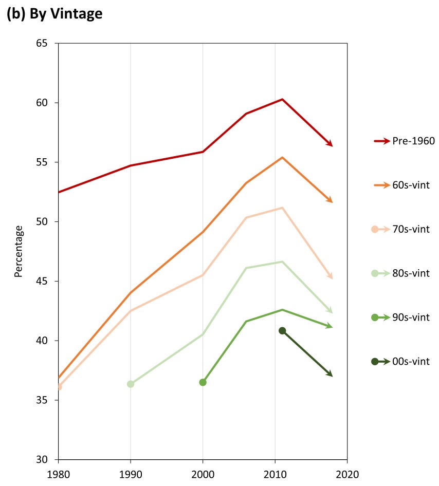
We can see how filtering works by looking at correlations between building age and occupant incomes or rents. Myers and Park (2020) use US census and ACS data to plot the share of below-median-income households living in rental buildings, separately by building vintage (construction year); see their Figure 4b below. As expected, when we compare across vintages, older buildings have more lower-income residents. Moreover, for each vintage the share of lower-income residents is increasing with time (and age) until 2011, then starts to decrease. This shows that filtering depends on the broader housing market: when housing supply is adequate, homes filter down; but when we face a shortage, homes filter up. Filtering is an outcome of housing supply and demand.
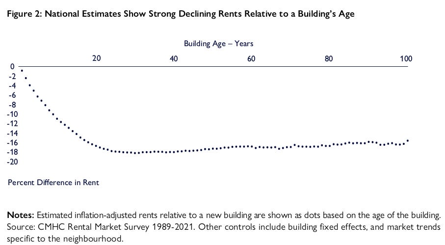
This CMHC report on rental apartments estimates how much rents decrease relative to a new building (see their Figure 2 below). As you would expect, older apartments have lower rents compared to new apartments, with the full effect occurring within 20 years. Note that this relative effect holds even if rents are increasing overall, because people have higher willingness-to-pay for newer buildings with new materials and construction techniques.2 It would be useful to see this graph split by metro area, where we expect a flatter graph in supply-constrained cities like Vancouver and Toronto, as demand increases bid up rents of older buildings.
Estimates of the filtering rate
While theoretical studies of filtering date back at least to Sweeney (1974), the first paper to directly estimate filtering rates was Rosenthal (2014) (published), using data from the American Housing Survey (AHS) over 1985-2011. He uses a repeat-income model, where we compare incomes for successive occupants of the same home. Filtering is measured as the change in occupant income at turnover.3 This is a direct measure of filtering, whereas previous estimates were indirect, using hedonic regressions of rents on age.4 Note that this method assumes that home characteristics (aside from depreciation) do not change between occupants.
Rosenthal’s main result is that housing filtered down at a rate of 1.9% per year over the study period. This implies that an arriving occupant of a 50-year-old home will have an income 60% lower than an occupant of a new home. Rental apartments filter down faster than owner-occupied homes, and owned homes transition to the rental market, which amplifies the overall filtering rate.
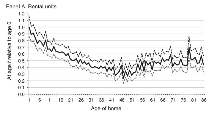
I plot his Figure 1a below, showing inflation-adjusted relative income against age for rental homes. The y-axis is the percentage difference in occupant income for a given home age compared to a new home. Here the filtering rate is the slope of the curve. For this time period, rentals clearly filtered down, with arriving occupants having lower income than initial occupants. (The graph for owner-occupied homes also shows down-filtering, though less pronounced.) The curve increases after age 50, probably due to survivor bias, as higher-quality homes are more likely to avoid demolition and stay in the dataset.
Rosenthal also uses simulations to test for heterogeneity in filtering across census regions, and shows that filtering rates are smaller when price growth is higher, notably in the New England and Pacific regions. Overall, we can say that over 1985-2011, housing supply was not overly constrained, so supply was able to keep up with demand, and homes were occupied by lower-income families as they aged.
But Liu et al. (2022) (published, working paper) shows that this conclusion does not hold after 2011. They study owner-occupied homes with Freddie Mac-funded mortgages over 1993-2018, and extend Rosenthal (2014) by testing for heterogeneity in filtering rates across geography and over time. They estimate a filtering rate around zero over 2012-2018, suggesting that supply constraints started to bind during this period, raising prices and inducing buyers of new homes to instead compete for the stock of old homes. When the housing market changed, the indicator changed.
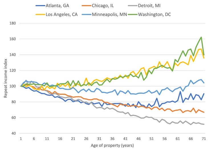
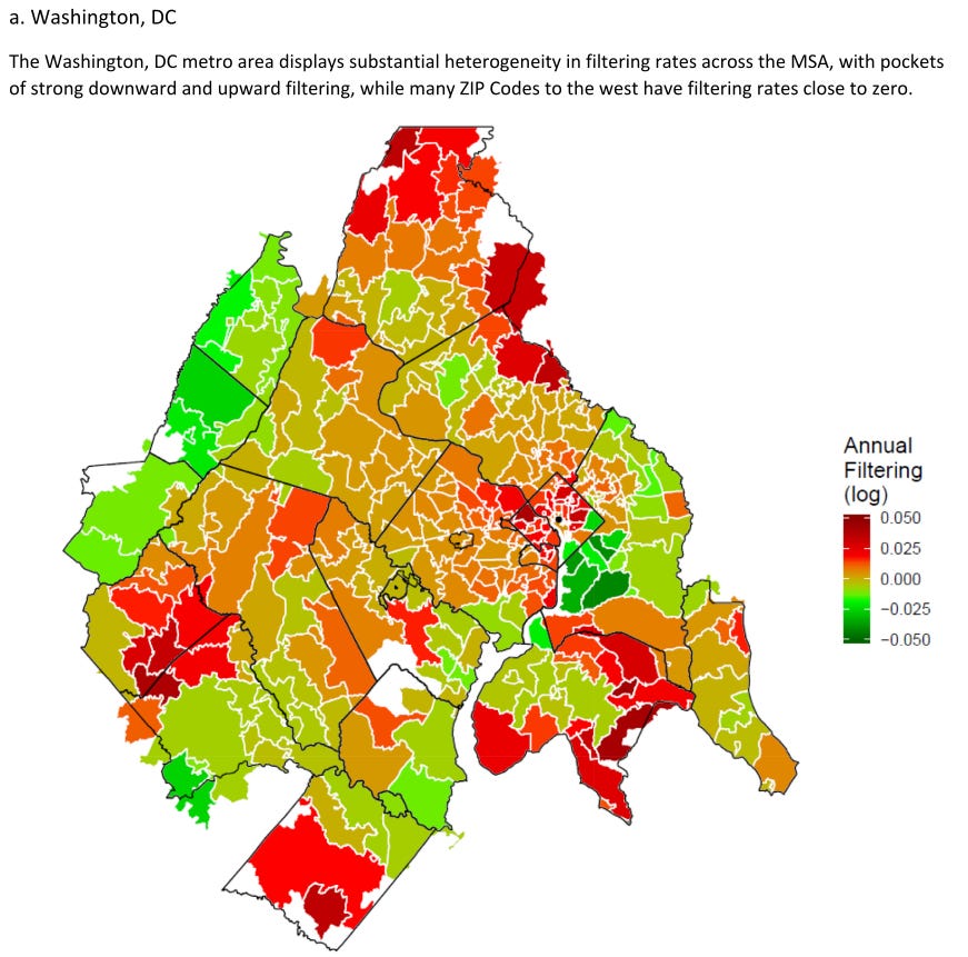
Liu et al. also find that filtering rates vary widely across metro areas, with up-filtering in LA and DC and down-filtering in Detroit and Chicago (see their Figure 2 below). As the filtering rate is an indicator for the housing market, this is consistent with regional housing markets performing differently. Restrictive zoning in LA means that supply can’t keep up with demand, so newcomers tend to be richer than current residents.
Lastly, they investigate within-metro heterogeneity in filtering rates (see their Figure 6a below). For instance, Washington DC has neighborhoods with strong down-filtering and neighborhoods with strong up-filtering. This illustrates how housing markets can vary across neighborhoods within the same city.
Spader (2025) (published, working paper) also extends Rosenthal (2014), this time using the same AHS data over a longer time period (1985-2013 and the new 2015-2021 sample). As with Liu et al., Spader finds down-filtering over 1985-2013, but up-filtering over 2015-2021. Again, this is consistent with a worsening housing shortage starting after the Great Recession.
Kindstrom and Liang (2024) (working paper) studies filtering in Sweden, using register data on all residents over 1990-2017. They don’t use a repeat-income model, but instead study how a building’s average income (relative to the national average) varies with building age. They find that, on average, a building’s relative income decreases by 14% (from 1.12 to 0.96) over 50 years. This is much smaller than the income decay of 60% in Rosenthal (2014), which is partly explained by lower inequality in Sweden.
Kindstrom and Liang report several other findings. First, adjusting for renovations leads to a much steeper filtering function, with relative income decreasing by 24% (from 1.12 to about 0.85) over 50 years. Second, it takes about 30 years for buildings to reach a representative income distribution, with equal shares of residents by income quartiles. Third, income decays faster in rental apartments compared to owned apartments, which in turn have faster income decay than detached houses.5
Hansen and Rambaldi (2025) (working paper) study filtering using data from the census of home transactions in Victoria, Australia over 2011-2016. They also use a different method than the repeat-income model, since they have data on buyer and seller income from the same home sale. This allows them to measure contemporaneous relative income as the ratio of buyer to seller income.6 They define the marginal filtering rate as the change in relative income with respect to age, and find up-filtering over this period, suggesting that supply constraints are binding.
Hansen and Rambaldi directly estimate the effect of supply constraints on filtering rates, using the share of development applications refused by local councils and a 2014 policy change partially removing council discretion. They find that higher refusal rates lead to more up-filtering, and that setting the refusal rate to zero implies a negative filtering rate (i.e., down-filtering). Since supply constraints drive price growth, removing those constraints would reduce prices and result in buyers having lower incomes than sellers.
Policy relevance
Rosenthal frames his paper as addressing the debate over housing vouchers vs. construction subsidies (e.g., LIHTC). If homes filter down to low-income families, Rosenthal argues, then we can provide subsidized housing by offering vouchers that families can use to access these low-price homes, as opposed to directly providing non-market subsidized housing.
This framing is odd. We don’t need to know filtering rates to judge whether vouchers will fully cover housing costs; we can simply look at current market rents. If rents are low enough, then a large-scale voucher program is feasible. However, the filtering rate would be relevant for forecasting the stock of low-income housing to evaluate a voucher program over the long-term.
Misinterpretations
The existence of up-filtering is not evidence that housing markets don’t work, as some claim. Instead, it can simply mean that markets are constrained by zoning regulations, and that we need to remove those constraints. Remember that filtering is just another housing market indicator; saying that up-filtering is evidence against markets is like saying that high prices are evidence against markets.
Spader makes this mistake: "In these areas [with up-filtering], supplying affordable housing units may require lower reliance on market-rate units and greater reliance on production of new housing units through LIHTC, inclusionary zoning, and other strategies for producing new affordable units." (p.20) Again, up-filtering just means there was a housing shortage. The natural remedy to a shortage is to increase supply, i.e, upzoning to add more market-rate homes.
Similarly, it’s equally mistaken to think that new homes automatically filter down and become affordable. If supply is constrained, up-filtering occurs instead. Liu et al. write that “filtering rates are equilibrium outcomes rather than fixed deep parameters of an economy.” (p.24) It speaks volumes that they felt the need to include this sentence!
Rosenthal’s title is "Are Private Markets and Filtering a Viable Source of Low-Income Housing?" There are two problems here. First, filtering is an outcome, not a mechanism, so it’s misleading to describe it as a source of low-income housing. This is like asking if prices are a viable source of low-income housing. But prices are the outcome, not a mechanism. Second, it neglects context. Markets may provide low-income housing in some locations and time periods, but not others. A better title would be: "Were Private Markets a Viable Source of Low-Income Housing Over 1985-2011"?
Prices need to be quality-adjusted, since unadjusted prices already account for depreciation.
The slope could be positive if developers built new lower-quality units, where the reduction in quality outweighed depreciation of aging rentals.
In the AHS data we observe income only for new occupants, so we need two turnovers to define a change in income.
That is, a regression of prices on age and other home characteristics. Here “hedonic” means utility, derived from the Greek for “pleasure”.
Since they use average building income, they can decompose by movers and stayers. By definition, the repeat-income method focuses on families who move into a home, and asks whether a home is occupied by poorer families over time. Since this is a descriptive exercise, the counterfactual is not well-specified. For example, if rising demand leads a young professional to stay in their home instead of moving out, then down-filtering was prevented; in a sense, this is up-filtering, since the home is occupied by a richer resident. In general, we have to be careful with causal interpretations.
Note that the repeat income method measures buyer income at consecutive transactions. Sellers could have systematically different income than buyers; for example, if sellers are retirees and buyers are young professionals, then up-filtering is expected.
Does the substantial heterogeneity in filtering rates within Washington DC MSA suggest that areas within the city, even neighbourhoods side by side, had significantly different supply constraints?
Is that the right interpretation of that heterogeneity?
That seems to be how you've interpreted heterogeneity between cities. So I'm assuming it holds within cities too.
Or is there some other interpretation of that heterogeneity, for example, differential demand growth between neighbourhoods (as some gentrify and others do not) leading to more up-filtering in neighbourhoods with faster-growing demand?