Gentrification and displacement

New housing enables rich people to move in without displacing the poor

When demand to live in a city is increasing, should we allow densification so that the supply of housing can keep up? The case for allowing density is straightforward: given that rich newcomers are moving in, getting them to live in new homes means they won’t outbid residents for the existing housing stock. When supply increases enough, it absorbs the new demand so that rents and prices stay flat. Hence, increasing housing supply leads to gentrification (richer people moving in) without displacement (poorer people moving out).

And we have research from England, Switzerland, and the US backing this up. What happens when the same demand increase hits areas that allow vs. block new housing? In places where supply cannot keep up with demand, these studies find that housing prices grow faster, they become gentrified, and displacement risk increases. This is what the standard supply and demand model predicts.

But constructing new apartment buildings could also improve neighborhood amenities and attract richer residents. If more supply brings nicer stores and cafes, then it will induce a secondary increase in demand. And if this “induced demand” effect is larger than the supply increase, then rents could rise overall. On this view, rents and displacement risk are lower when we respond to a demand increase by blocking new density.

We can empirically test for induced demand. If new buildings bring amenities that make the neighborhood more desirable, we should see higher rents and displacement risk nearby. However, multiple studies report that adding new apartment buildings reduces rents and displacement in the same neighborhood. Moreover, these papers show that naive correlations between construction and rents do not capture causation, because developers tend to build in already-gentrifying areas.

Demand increases lead to gentrification and displacement

There are several papers studying the effects of increases in housing demand, looking at effects on prices, rents, and evictions. The key is to compare the same demand increase across areas with more- and less-constrained housing supply. Since supply constraints prevent new homes from absorbing the increase in demand, we should see a larger increase in prices and rents in areas with constrained supply.

Hilber and Vermeulen (2016) (working paper, published) tests whether increases in housing demand have a larger effect on prices when supply is more constrained. They use panel data on 353 Local Planning Authorities (LPAs) in England over 1974–2008, with price data on detached houses and townhomes. To measure supply constraints, they look at how often the local government rejects residential projects with 10+ homes (the ‘refusal rate’). One problem is that the refusal rate can be a biased proxy: if developers know an application will be rejected, they won’t apply in the first place; so observed refusals could understate how much a local government restricts supply. The authors address this by using a 2002 permitting reform as a change in actual restrictiveness.

Measuring housing demand is also tricky. Average income is often used as a proxy, but observed incomes are partly determined by whether an area allows enough housing so that new workers can move in. (We say that income is ‘endogenous’ to supply constraints.) Instead, Hilber and Vermeulen use a demand measure based on a city’s industry mix in 1971 and national industry employment growth afterwards. If your city had industries that boomed nationally, we’d predict higher housing demand. This ‘Bartik demand shifter’ allows us to define an increase in housing demand that is consistent across cities, regardless of actual supply constraints.¹

The main results are from a regression of log prices on the interaction of the demand shifter and supply constraints. They find that a demand increase raises prices much more in cities that block new housing. Specifically, a 1 standard deviation increase in supply constraints raises the price-demand elasticity by around 0.7 (see their Table 5). In other words, when we make supply more constrained, the effect of a demand shift on housing prices becomes stronger. To give an intuitive interpretation, they use a counterfactual exercise: if regulatory supply constraints were removed entirely, housing prices would fall by about 16% (see Table 7).

Buchler et al. (2025) (working paper, published) repeats the same exercise using data on prices and rents in Switzerland over 2010-2021. They measure supply constraints using an index of density restrictions based on assessments of local officials, and use a Bartik shifter as the change in housing demand. As with Hilber and Vermeulen, they find that supply constraints amplify the effect of demand growth on prices and rents. For a given demand shift, price growth is 8% higher and rent growth is 13% higher when density is restricted at the 75th percentile compared to the 25th percentile. In an earlier study on US metros, Saks (2008) (working paper, published) also finds that demand increases lead to bigger increases in housing prices when supply is more constrained.

Asquith (2025) (working paper) studies the effect of housing demand increases on evictions and the stock of rent-controlled housing in San Francisco over 2004-2013. He uses the rollout of private shuttles run by tech companies as a demand shock, where a new shuttle stop in a neighborhood drives increased local demand. For example, Google employees moved to San Francisco after their IPO made them rich enough to buy a home in the city and take the shuttle to the office in Mountain View.

In preliminary results, he finds that the demand shock caused around 40 duplex landlords per year to evict their tenants and withdraw their rentals from the rent-controlled housing stock. This occurs even despite regulations strongly disincentivizing such withdrawals: under the Ellis Act, landlords have to give up two years of rental income and face ten years of restrictions before they can exit the rental market.² Basically, renting or selling to tech workers was actually so lucrative for landlords that it was worth paying these regulatory costs.

Since San Francisco builds very little housing, we can interpret these results as showing what happens when housing demand increases and supply is prevented from keeping up. This is low-density gentrification, where rich people move into the neighborhood without an increase in density. If housing supply was more elastic, demand from new tech workers would have been absorbed, instead of spilling over into the existing rental market. Hence, Asquith shows how evictions and displacement are caused by restrictions on housing supply.³

Future research

Economists find it obvious that demand increases cause higher prices, so there are few studies on this question. But since laypeople are skeptical that housing supply matters, it would be helpful to have more research showing what happens after an increase in housing demand. A US study could extend Hilber and Vermeulen by using the Baum-Snow and Han (2024) supply elasticities to show that a demand shift leads to larger price increases in low-elasticity neighborhoods where zoning prevents supply from keeping up. Another approach is to show the ‘demand cascade’, where increases in high-end demand cause richer locals to downgrade, thereby increasing demand in the low-end market. For example, use a Bartik shifter for college-educated workers (compare Edlund et al. 2022) and show that prices and rents rise for both high- and low-end housing (or if using age to measure quality, for both new and old homes). With data on residential addresses, we could study the effect on displacement (evictions or moving to a poorer neighborhood) and gentrification (in-migration from a richer neighborhood). And with data on families, we could show that higher demand leads to larger households via doubling-up.

Increased supply causes gentrification without displacement

If supply constraints lead to higher rents and displacement in the face of growing demand, what happens when we allow supply to keep up with demand? A recent literature studies the local effects of new housing supply. These papers use the construction of new apartment buildings as the treatment variable, and test for spillover effects on rents in other buildings in the same neighborhood.⁴ As we’ll see below, developers build in areas where demand was already rising. So just comparing neighborhoods with vs. without a new building will give us a biased answer. To estimate the causal effect of new construction, we need a proper control group that follows the same trends as the neighborhood with the new building. Moreover, we should think of these papers as studying what happens when new apartment buildings are constructed in the context of rising demand.

The new buildings increase the supply of homes, which has a negative effect on rents. However, new buildings don’t just change the housing stock, they also change the neighborhood. If a new building improves local amenities and makes the neighborhood more desirable, then there is an induced-demand effect that increases local rents (while reducing demand and rents elsewhere).⁵ On the other hand, higher density leads to more congestion and can make the neighborhood less desirable (a deterred-demand effect). We estimate the net effect of the supply and amenity channels, and the evidence shows that the supply effect dominates: even if neighborhoods do become nicer, we still see a net decrease in rents.⁶

Asquith, Mast, and Reed (2023) (working paper, published) is the key paper in this literature. They study the local effects of large market-rate rental buildings, using data from 11 cities over 2010-2019.⁷ To capture amenity effects, they focus on ‘pioneer’ buildings, defined as the first new building in a neighborhood since 2010. They also limit the sample to low-income areas, meaning census tracts with median household income below the metro median. They use Zillow rental data from 2013-2018 and Infutor migration data from 2011-2017.

The paper uses multiple empirical approaches based on a difference-in-differences strategy, which compares a treatment and control group before and after a treatment takes effect. Their most persuasive method compares neighborhoods with new buildings completed in 2015-16 (treatment group) to neighborhoods with buildings completed in 2019 (control group). Both groups have a new building at some point, so we are making an apples-to-apples comparison. Note that they are comparing the treatment and control groups over the period (2013-2018) before the control neighborhoods have a building completion. They define the treatment area as a 250m (820ft) ring around the new building, capturing an area of 1-2 city blocks. The median new building increases the rental stock within 250m by 37%, so they are capturing a large supply shock.

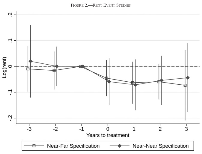
The main results are in the Figure 2 event study (see below, ‘Near-Near Specification’), with the coefficients showing the effect relative to the control group. They find an immediate drop in rents in the year of completion, staying around 6% lower for three years. The flat pre-period coefficients (to the left of year 0) support the ‘parallel trends’ assumption that the treatment and control groups follow similar trajectories before the building is completed. Across all specifications, they find a 5-7% decrease in rent, translating to $100-$159 monthly.⁸

They also find consistent effects on in-migration. Their Figure 4 shows that in-migrants to the neighborhood with the new building are more likely to move from poorer neighborhoods, which makes sense if rents are falling nearby.⁹ Hence, even in low-income neighborhoods where new buildings may induce demand by improving amenities, the net effect of new market-rate housing is to decrease rents.¹⁰

Li (2022) (working paper, published) does a similar exercise, studying the effect of new residential high-rises in New York City over 2003-2013. Her sample includes high-rises with 7+ storeys, with data on 916 completions. She looks at the spillover effect on rents of existing residential buildings within a 500ft radius.¹¹ Her difference-in-differences method compares neighborhoods that have a new high-rise completed nearby, with variation in timing of completion. The average building increases the total housing stock nearby by 9.4%.¹²

Her main result is that a 10% increase in housing units nearby reduces rents by 1% (see Table 2). The event study in Figure 5 shows that this is not driven by differential trends in treated neighborhoods before completion, and that the effect becomes more negative over time. Li also finds suggestive evidence that new high-rises improve amenities, with an increase in new restaurants. So even if improved amenities lead to increased demand, the effect is outweighed by the increase in supply, since we observe a decrease in rents.

Rollet (2025) (working paper) extends Li’s dataset and runs the same test in New York City over 2003-2021. Rollet makes a few different modelling choices: he uses floorspace while Li uses housing units; his sample is based on new residential buildings with a large percentage and absolute increase in floorspace¹³, resulting in 290 completions; finally, Rollet defines an observation as a 500ft neighborhood disk around a new building, instead of using parcel-level data. He also improves on Li (2022) by using a modern event study estimator that avoids using already-treated units in the control group. In preliminary results, Rollet finds that building completions lead to a steady decline in nearby rents, which continues 10 years afterwards. He reports that a 10% increase in floorspace reduces rents by 4.2%. This effect is much larger than Li’s, and can be explained by differences in the study designs.¹⁴

Pennington (2025) (working paper) is another recent paper studying the local effects of supply increases. She uses serious building fires in San Francisco over 2013-2017 as a source of new construction, and estimates the effects of new buildings on rents, displacement, and gentrification. She measures rents using Craigslist data and uses Infutor address data to define moves. Displacement is defined as moving to a zipcode with at least 10% lower median income, while gentrification means higher-income newcomers moving into the neighborhood. Hence, gentrification can occur without displacement. In preliminary results, Pennington finds that new market-rate construction reduces rents and displacement and increases gentrification.¹⁵

Finally, Brunåker et al. (2024) (working paper) use population register data from Sweden over 1991-2017 to study the effect of new market-rate buildings in poor neighborhoods on gentrification and displacement. They focus on large co-ops (equivalent to condos) with more than 100 residents; following Asquith et al., they restrict the sample to ‘pioneer’ buildings, with no similar buildings in the same neighborhood in the previous 11 years. This gives 76 new buildings in neighborhoods with bottom-quartile income. They use a stacked difference-in-differences method, selecting control observations in the same municipality with similar income rank. As with Pennington, they find gentrification without displacement: rich people move into the new buildings, but there is no reduction in the rental stock and no out-migration from the neighborhood.

Developers build in already-gentrifying neighborhoods

Asquith, Mast, and Reed show that there is a strong selection effect for the location of new buildings: developers build in neighborhoods that are already gentrifying. In Table 2, they compare neighborhoods with versus without new housing over 2000-2010, the pre-construction period. The areas with new construction after 2010 had higher income growth (11% vs -1%), higher growth in college-graduate share (12% vs 5%), and slightly higher rent growth (19% vs 16%). Hence, a simple comparison of new construction and rents will show a positive correlation, because developers choose to build in neighborhoods with rising rents. But as we’ve seen, a proper causal analysis finds that new supply reduces rents.

Li also shows that developers choose to build in areas with rising rents. When we compare treated parcels (with a new high-rise nearby) to control parcels, we see a pre-trend in rents prior to completion of the new building (see her Figure 4). This shows that rents were already rising in the treated neighborhood before the new building was completed. Hence, we have strong evidence against the naive view that infers causation from the correlation between new construction and higher rents.

Metro-wide effects

Beyond local effects of new supply, we also have evidence that increasing housing supply reduces rents across the entire metro area. Mense (2025) (published) uses variation in new construction driven by wintry weather in Germany. He reports that a 1% increase in new completions lowers average rents by 0.19%.¹⁶ He studies heterogeneity by housing quality, finding a 0.13% rent decrease in the bottom decile of quality, and a 0.28% decrease in the top decile. Hence, housing supply decreases rents at the metro level, with an additional local effect at the neighborhood level.

How much density is needed to offset displacement?

Even if new housing supply reduces rents nearby, it may still cause displacement directly if construction requires tearing down cheap old homes and evicting renters. So while zero-displacement projects are unambiguously good, projects that displace renters through redevelopment are less clear-cut. This raises the question: what is the level of densification needed for these opposing effects to cancel out? That is, when tearing down one old home, how much do we need to densify to reduce rents enough to offset the loss of the old home? We want to know the breakeven level of densification.

Vacancy chain studies offer one answer to this question. They find that each new market-rate home frees up 0.6 homes in below-median-income neighborhoods. So the new building needs to be at least 1/0.6 = 1.67x bigger (in number of units) than the old building to maintain the stock of cheap homes. Note that the offsetting occurs at the metro level, not at the neighborhood level.

Nathanson (2025) (working paper) does a stricter version of this exercise, where we redevelop a home in the bottom decile of quality, replacing it with top-decile homes. He asks how much we need to densify to maintain the price of bottom-decile housing, with the price effect of new top-decile supply offsetting the decrease in the bottom-decile stock. He finds a breakeven threshold of 5x, so the new building needs to have at least five times more units. Note that the vacancy chain multiplier is from looking at below-median instead of bottom-decile, so naturally that threshold is smaller.

1. Think of ‘demand shift’ as a shift in the demand curve. The Bartik shifter for a given city is a weighted average of national employment growth by industry, weighting by the industry’s initial share of employment in the local economy. This is also known as a shift-share instrument.

2. In California, landlords can use the Ellis Act to evict all of their tenants and remove their building from the rental market, but only under strict conditions, including: paying relocation costs to tenants; not renting the property for two years; and offering right of first refusal to the original tenants at their original rents (plus allowable increases) for the first five years. All restrictions are removed after ten years.

3. Were the restrictions on Ellis evictions just not strong enough? Suppose landlords were required to forego five years of rental income (instead of two). This would reduce evictions, but doesn’t address the root cause of increased demand to live in San Francisco. So we’d expect landlords to find other margins to capture market-rate rents, or to disinvest and reduce building maintenance as returns are increasingly below-market.

4. These papers measure local effects on rents, and cannot measure metro-wide effects, since the control group is in the same metro and experiences the same metro-wide effect. Hence, the papers underestimate the total effect of new supply on rents. Note that classic urban economics models assume perfect spatial substitutability within a metro, so a supply increase should have the same price effect across the metro. In other words, the local effect should be zero. The nonzero effect in this literature is evidence against this assumption.

5. Since induced demand means drawing in residents from elsewhere, there is no straightforward policy implication. Increased demand in one neighborhood means reduced demand elsewhere. So even if residents near the new building are worse off due to higher rents, residents in the origin neighborhoods of the movers (from which the demand was induced) are better off. So at first glance, induced demand has no net welfare effects. This could change if the induced demand represents second homes, so there is a net increase in demand, rather than a reallocation; or if the destination neighborhoods have higher welfare weight due to being lower-income.

Also notice that induced demand involves a feedback loop: shifting the short-run supply curve leads to a shift in the demand curve, which triggers another increase in supply, and so on. Proponents of induced demand do not seem to recognize this.

6. How does induced demand matter for the demand shock papers above? One possibility is that amenities improve as a function of quantity supplied, so there’s a bigger induced demand effect in the less-constrained area (compared to the more-constrained area). This would shrink the differential price effect (and in the extreme case, flip it). But the relationship between amenities and housing quantity is likely more complicated, since suburban sprawl is generally not seen as an amenity.

7. Atlanta, Austin, Chicago, Denver, Los Angeles, New York City, Philadelphia, Portland, San Francisco, Seattle, and Washington, DC.

8. They don’t observe the total housing stock, so they can’t calculate an elasticity (the percentage change in rents for a 1% change in units).

9. Though note that they do not observe individual income, so these movers could be richer people in poorer neighborhoods.

10. The decrease in rents could be partly explained by deterred demand via congestion or disamenity effects. They test for a doughnut-shaped effect, where congestion occurs within 250m and there is a positive amenity effect in the 250-600m ring. The results are inconclusive.

11. She has data on building-level rents, which adds noise compared to unit-level rents.

12. Asquith et al. use buildings that increase the rental stock by 37%. Since they don’t observe ownership housing, it’s not clear whether their supply increase is larger than Li’s. The supply increases are equal if the AMR share of rental housing is 0.25.

13. Within a 500ft radius, the new building must increase floorspace by >10% and by >20,000sqft.

14. First, Rollet uses a longer treatment window, capturing effects ten years after completion (while Li uses five years); since the effect size increases over time, he will mechanically measure a bigger effect. Second, since he uses floorspace while Li uses units, if the new buildings have smaller units, a 10% increase in units corresponds to a <10% increase in floorspace. So Li might be evaluating (say) a 5% increase in floorspace, which generates a smaller elasticity. Third, Rollet uses larger buildings, which could have a smaller amenity effect through increased congestion, leading to a larger effect on rents.

15. This is the most extreme case for difference-in-differences: the number of fire-induced buildings nearby is a continuous treatment variable with a time-varying treatment dose. Modern estimators that can handle this case have become available only recently.

16. Average new completions (flow) are 0.48% of the total stock.